A Model to Quantify the Degree of Customization (DoC)

Customizing packaged software products, like ERP and CRM systems, has an adverse effect on their upgradability and maintainability. Typically a company acquiring a packaged product wants to balance out the investment (ROI, TCO) with just enough adjustments that are required to make the product fit the industry or business specific aspects (usability) so the company can retain its competitive advantage.
Making too many adjustments voids the purpose of investing in a packaged product. A better solution would be a bespoke software in that case. Not enough adaptation and sticking to the out of the box functionality reduces the ability of a company to serve its clients and by that the usability of the packaged product. So there is a sweet spot for every company with the right amount of adjustments.

In order to determine this sweet spot a company must be able to determine the degree of adaptation that was applied. Quantification is difficult but not impossible as we will show in this document. Once quantified it allows to monitor the current state and trend in the adjustments that are made to the original packaged product.
The original paper I wrote on this model you can download here:
The Degree of Customization (DoC) model is a way to quantify the amount of adaptations to a software product. It expresses the degree as a percentage where 0% indicates the out of the box product and where 100% indicates a fully bespoke product.

The DoC is based on three axes:
- The count of the adaptations
- The impact of the adaptations
- The size of the adaptations

The DoC determines the degree for the building blocks comprising the software. What these building blocks are and the level of granularity is up to the company to determine. However, the granular finer and more exhaustive a list of building block is defined the more detailed and accurate the DoC can be measured.
As a solution to define the building blocks we propose the traditional RICEFW bottom-up approach that is also being used in project estimations. Aligning to the same factors that are used in project management and architecture makes the model practical and reduces the effort to gather the necessary information. This approach starts with creating an inventory of components that potentially can be adapted. These components are:
- Reports (reports)
- Integrations (interfaces)
- Business logic (conversions)
- Data Entities (enhancements)
- User Interfaces (forms)
- Business processes (workflows)
If a course grained DoC is sufficient only the business processes will be taken into account. For a fine grained DoC calculation also the other components, that are used to realize the business processes, are taken into account i.e. user interface, data entities, business logic, integrations and reports.
To calculate the DoC a four-step approach is proposed:

- Identify
- Categorize
- Size
- Analyze
Step 1: Identify


In this step an inventory is made of the components that are part of the packaged software. To calculate a correct DoC it is important to have an exhaustive list. The level of granularity is discretionary but for the selected level the list must be exhaustive.
Some options for the granularity i.e. DoC domains:
- High-Level DoC: business processes
- Business DoC: High-Level Doc, business logic and data entities
- Internal DoC: Business DoC, user interface and reports
- External Doc: interfaces
- Detailed DoC: Internal Doc, External DoC
This inventory forms the frequency (count) axes of the model.
Step 2: Categorize


Once the inventory is created the level of adaptation per component must be determined. To achieve this, five categories are used and every component must be assigned to a category:
- Cat 1: Out-of-the-box used component
- Cat 2: Component is adapted through configuration
- Cat 3: Component is adapted through no-code extensions
- Cat 4: Component is adapted through coded extensions
- Cat 5: Component is adapted through bespoke customization
Each category will be assigned a customization impactor factor later on (α-function), to calculate the DoC. The category forms the impact axes of the model.
Step 3: Size


An adaptation of a small component has less impact than the adaptation of a large component. To make an accurate calculation we have to correct the component’s impact based on the component’s size. To achieve this T-shirt size categories are use:
- Size 1: Small
- Size 2: Medium
- Size 3: Large
The size definitions is again discretionary but a fix set of definition must be used using quantifiable characteristics. Typical for the characteristics is that they evolve exponential across the size buckets. The size bucket will be used later on as weighing factors (β-function) for the components based on the customization size.
Size examples per component inventory categories:
| S | M | L | |
| Reports (reports) | Standard formatting, fixed filtering, 5-10 columns | Standard formatting, ad-hoc filtering, 10-25 columns | Custom formatting, ad-hoc filtering, > 25 columns |
| Integrations (interfaces) | 1 entity, 5-10 fields, ad-hoc, internal communication | 2 entities, 10-25 fields, messaging, internal-external communication | > 2 entities, > 25 fields, orchestration, external communication |
| Business logic (conversions) | 1 entity data mappers, 1 backend operation, no data triggers, no process triggers | 5-10 entity data mappers, 5-10 backend operation, mappers, data triggers no process triggers | > 10 entity data mappers, 10 backend operations mappers, data triggers process triggers – |
| Data Entities (enhancements) | No custom entities, 5-10 attribute extension | 5-10 custom entities, 10-25 attribute extension | > 10 custom entities, > 25 attribute extensions |
| User Interfaces (forms) | 1 data source, 1 entity, 5-10 fields, basic data representation, text input and button UI controls | 1 – 2 data sources, 1-5 entities, master-detail representation, graphical UI controls | > 2 data source, > 5 entities, custom representation, complex graphs and 3D controls |
| Business processes (workflows) | 5-10 process steps, no orchestration, no external interactions | 10-25 process steps, orchestration, 1 – 2 external interactions | > 25 process steps, orchestration, > 2 external interactions |
Step 4: Analyze

To calculate the DoC following factors are used:
| Category | Customization Impact α-function |
| Cat 1: Out-of-the-box | 0,00 |
| Cat 2: Configuration | 0,25 |
| Cat 3: No-code extensions | 0,50 |
| Cat 4: Coded extensions | 0,75 |
| Cat 5: Bespoke customization | 1,00 |
| Size | Customization Size β-function |
| Size 1: Small | 1 |
| Size 2: Medium | 2 |
| Size 3: Large | 4 |
Next the DoC is determined using the following formula:
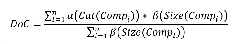
To calculate the DoC, a size-weighted average is calculated of the impact of all the inventoried components
The DoC calculation will return a percentage that identifies where on the spectrum of out-of-the-box to fully customized the adaptations to the packaged solutions lay.

Conclusion
Once determined the DoC level, the changes to the DoC can be monitored over time.
As rule of thumb a DoC of 50% is considered an acceptable level.
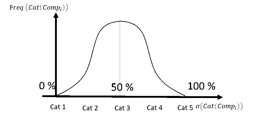
This means on average there are as many no-, low-impacting and no-code impacting adaptations as there are coded and bespoken adaptations. Going beyond this threshold of 50% it means that the usefulness of a packaged product becomes low compared to build fully bespoke from scratch.
